4 minutes
Sample size and Power calculation for Bland-Altman method comparing two sets of measurements in R
Motivation
I was recently approached by a PI to complete sample size and power calculations for Bland-Altman agreement assessment using the Lu et al (2016) formulation. The goal of this short tutorial is to demonstrate how to perform quick sample size calculations in R following Lu et al (2016).
Limits of agreement (LOAs)
Let \(D\) be the random variable representing the difference between two sets of measurements \(X\) and \(Y\). For a sample of \(d_i = x_i - y_i\), \(i=1,\dots,n\) with mean \(\bar{d}\) and standard deviation \(s_d\), the \(100(1- \gamma)\%\) LOAs can be calculated as \(\bar{d} \pm z_{1-\gamma/2}s_d\), which yields an upper limit and a lower limit of LOA.
The \(100(1- \alpha)\%\) confidence interval estimation of the \(100(1- \gamma)\%\) LOAs can be obtained following
\[Lower bound = (\bar{d} - z_{1-\gamma/2}s_d) - t_{1-\alpha/2, df=n-1} s_d \sqrt{\frac{1}{n}+\frac{z^2_{1-\gamma/2}s_d}{2(n-1)}} \] \[Upper bound = (\bar{d} + z_{1-\gamma/2}s_d) + t_{1-\alpha/2, df=n-1} s_d \sqrt{\frac{1}{n}+\frac{z^2_{1-\gamma/2}s_d}{2(n-1)}}. \]
We can proceed with sample size calculation by pre-specifying i) a desired confidence band/limit of the LOAs and ii) the two significant levels \(\alpha\) and \(\gamma\) (e.g. commonly set at 0.05).
The confidence interval of LOAs can be assumed symmetric. The decomposition of the type I and II errors of LOAs is shown in the figure below (taken directly from the paper). The two type II error terms, \(\beta_1\) and \(\beta_2\) can be calculated following a non-central t-distribution,
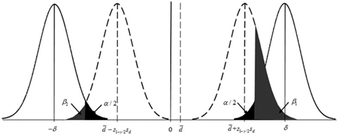 Figure 1, from Lu et al (2016).
where \(\beta_1 = 1 - probt[t_{1-\alpha/2, n-1}, n-1, \tau_1 ]\) and \(\beta_2 = 1 - probt[t_{1-\alpha/2, n-1}, n-1, \tau_2 ]\) and \(\tau_1\) and \(\tau_2\) are the two non-central distribution parameters. For mathematical details including the definition of \(\tau_1\) and \(\tau_2\) and the final power formula please see Lu et al (2016).
Power Calculation
For power calculation under a given sample size, we specify the following parameters
- \(\bar{d}\), mean difference between the two sets of measures
- \(s_d\), standard deviation of the difference
- \(\delta\), targeted clinical agreement limit
- \(n\), available sample size
- \(\alpha\), targeted confidence level of CIs of LOAs
- \(\beta\), targeted confidence level of LOA
Example 1. We have \(\bar{d} = 0.2\), \(s_d=1\), \(\delta=2.5\), \(n=203\) and \(\alpha = \beta = 0.05\). The following R code returns the power estimate using Lu et al (2016). Under this setting, the study has 80% power.
# attempt to verify Lu et al (2016) example;
# https://doi.org/10.1515/ijb-2015-0039;
mud = 0.2 #mean of difference;
sd = 1 #expected sd of the difference;
delta= 2.5 #targeted clinical agreement limit;
n = 203 #available sample size;

alpha = 0.05 # 95% confidence level of CIs of LoAs;
gamma = 0.05 # 95% confidence level of LoA;

# non-centrality parameter tau1 and tau2;
tau1 = (delta - mud - qnorm(1-gamma/2)*sd)/(sd*sqrt(1/n+qnorm(1-gamma/2)^2/(2*(n-1))))
tau2 = (delta + mud - qnorm(1-gamma/2)*sd)/(sd*sqrt(1/n+qnorm(1-gamma/2)^2/(2*(n-1))))

power = pt(qt(1-alpha/2,n-1), n-1, ncp=tau1, lower.tail = FALSE)+pt(qt(1-alpha/2,n-1), n-1, ncp=tau2, lower.tail = TRUE)

#return power estimate;
power
## [1] 0.8042332
Sample Size Calculation
Example 2. We can extend the code above to return power calculation giving a sequence of sample sizes. Let’s say we are interested to identify sample sizes corresponding to 70% and 90% power.
The R code below produces a simple power curve and returns the required sample size to reach 70%, 80% and 90% power.
# attempt to verify Lu et al (2016) example;
# https://doi.org/10.1515/ijb-2015-0039;
mud = 0.2 #mean of difference;
sd = 1 #expected sd of the difference;
delta= 2.5 #targeted clinical agreement limit;
n = seq(100,400,1) #sample size range between 100 to 400;


alpha = 0.05 # 95% confidence level of CIs of LoAs;
gamma = 0.05 # 95% confidence level of LoA;


# non-centrality parameter tau1 and tau2;
tau1 = (delta - mud - qnorm(1-gamma/2)*sd)/(sd*sqrt(1/n+qnorm(1-gamma/2)^2/(2*(n-1))))
tau2 = (delta + mud - qnorm(1-gamma/2)*sd)/(sd*sqrt(1/n+qnorm(1-gamma/2)^2/(2*(n-1))))

power = pt(qt(1-alpha/2,n-1), n-1, ncp=tau1, lower.tail = FALSE)+pt(qt(1-alpha/2,n-1), n-1, ncp=tau2, lower.tail = TRUE)

results<-cbind(n, power)

# view sample size and power table;
head(results)
##        n     power
## [1,] 100 0.5118853
## [2,] 101 0.5153101
## [3,] 102 0.5187459
## [4,] 103 0.5221911
## [5,] 104 0.5256439
## [6,] 105 0.5291028

# plot power curve;
plot(n, power, type = "l")
abline(h = 0.8, col = "red")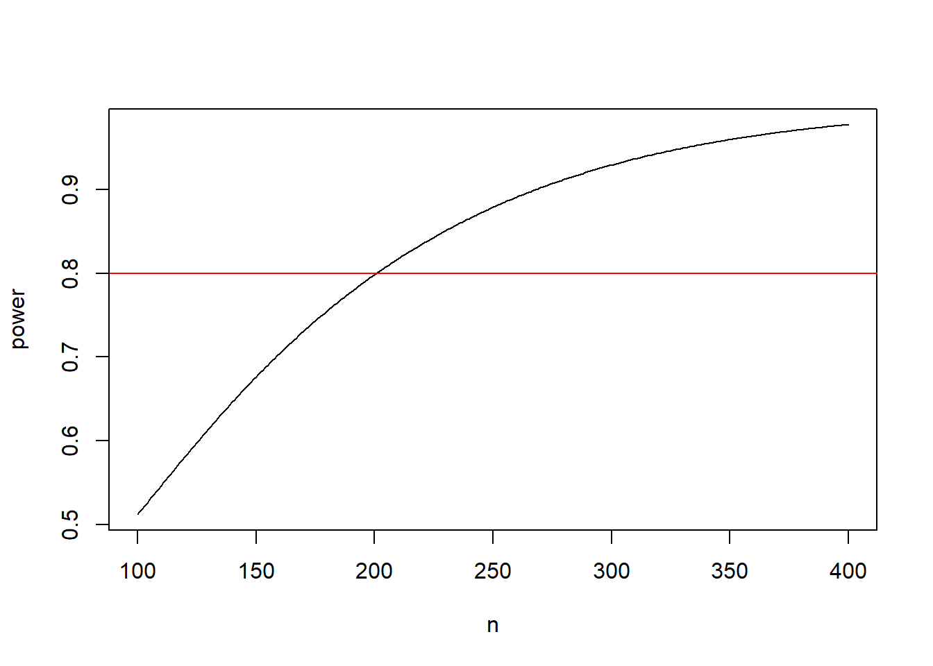
# return sample size at 70%, 80% and 90% power;
# for this calculation we select the sample size that yields the smallest value over the target power threshold.
rbind(results[min(which(results[,2] > 0.7)),],
      results[min(which(results[,2] > 0.8)),],
      results[min(which(results[,2] > 0.9)),])
##        n     power
## [1,] 159 0.7016833
## [2,] 201 0.8003178
## [3,] 269 0.9010620
The minimum required sample size to reach 70% power is 159 and minimum required sample size to reach 90% power is 269.
Bland-Altman agreement assessment sample size and power statistical consulting
750 Words
2021-08-07 (Last updated: 2022-05-03)
e8754b8 @ 2022-05-03