4 minutes
Creating static and interactive Nightingale rose diagram using ggplot and plotly in R
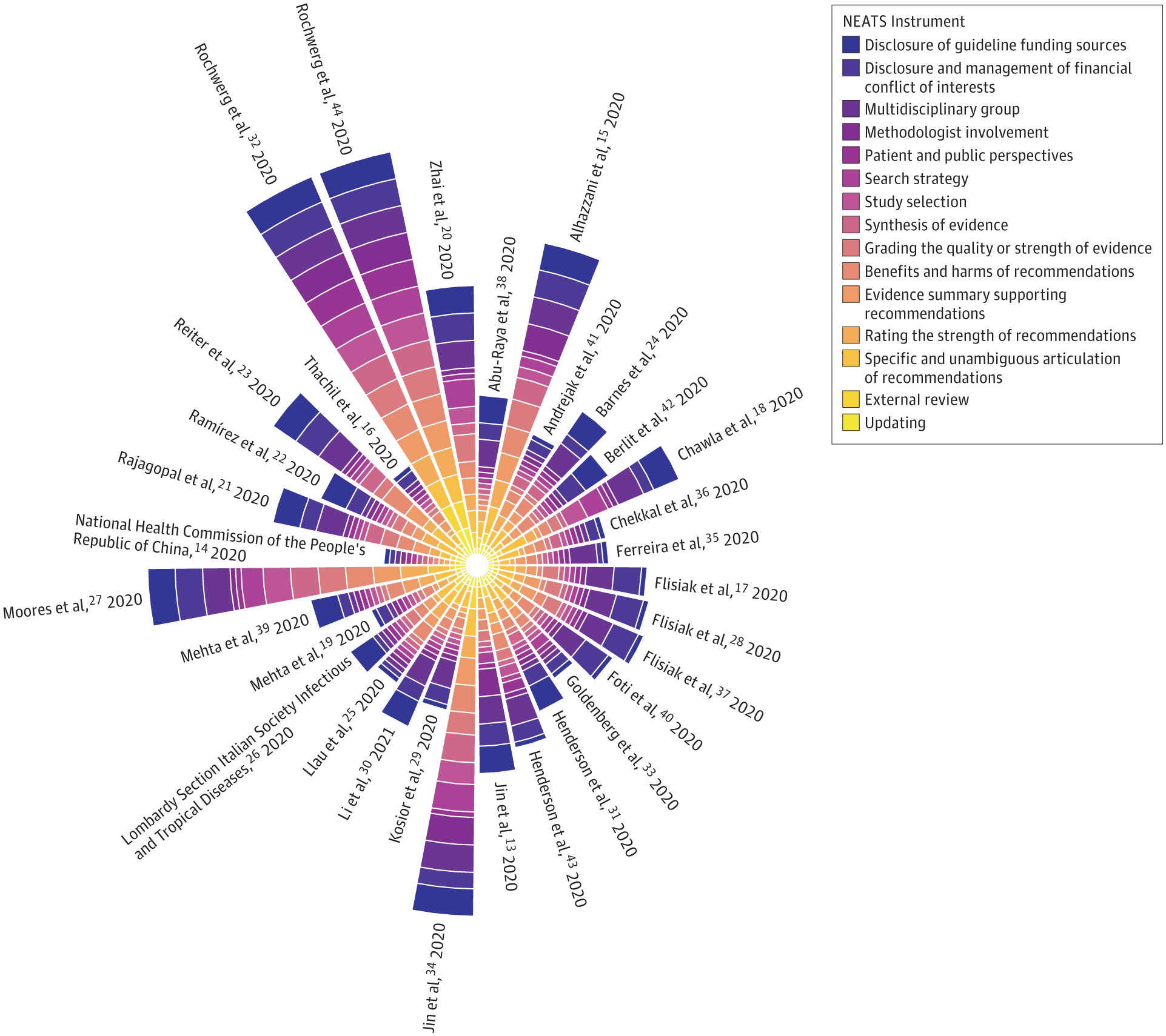
Example plot from Burns et al. JAMA Network Open (2021)
Creating Nightingale rose diagram using ggplot (static figure)
This plot is also called Wind Rose and Coxcomb diagram.
This diagram was developed by Florence Nightingale (1820-1910), a statistician, nurse and social reformer who was the foundational philosopher of modern nursing.
For demonstration purpose, I will simulate a simple data inspired by the example figure.
Suppose we have three variables in our data
- Year: 2016 to 2021
- Instruments of health: physical, mental and social
- my self-reported measure of health by instruments: a score between 1 and 5, where 5 represents the highest level of self-reported health
library(tidyverse)
library(DT)

set.seed(123)
dat <- tibble(
  Year = paste0("Y",rep(2016:2021, each=3)),
  Instrument = rep(c("physical","mental","social"),6),
  Score = sample(1:5, size = 3*6, replace = T))

dat %>% datatable(
  rownames = FALSE,
  options = list(
    columnDefs = list(list(className = 'dt-center',
                      targets = 0:2))))
we plot year as our rays (or rose petals) and instruments as stacked bars with height representing the scores.
Adding labels on top of each ray. This step requires we position the label using angle degrees.
library(viridis)

p <- ggplot(dat) +
  # Add the stacked bar
  geom_bar(aes(x=Year, y=Score, fill=Instrument), stat="identity", size=0.6, color="white") +
  scale_fill_viridis(discrete=TRUE, direction = 1, option = "C", name="Health Instrument") +
  ylim(0,15) + #using -1 as the lower bound to leave space in the centre of the polar
  coord_polar() +
  theme(
    panel.background = element_rect(fill = "white", colour = "white"),
    panel.grid.major = element_blank(),
    panel.grid.minor = element_blank(),
    panel.border = element_blank(),
    axis.line = element_blank(),
    axis.ticks = element_blank(),
    legend.position = "right",
    legend.text = element_text(size=18), #large font for website display
    legend.title = element_text(size=20), #large font for website display
    axis.text = element_blank(),
    axis.title = element_blank())

# Add labels on top of each bar
label_data <- dat %>% group_by(Year) %>% summarize(Tot=sum(Score))
angle= round(90 - 360 * (c(1:nrow(label_data))-0.5) /nrow(label_data),0)     # I substract 0.5 because the letter must have the angle of the centre of the bars. Not extreme right(1) or extreme left (0)
label_data$hjust<-ifelse(angle < -90, 1, 0)
label_data$angle<-ifelse(angle < -90, angle+180, angle)

p + geom_text(data=label_data, aes(x=Year, y=Tot+0.5, label=Year, hjust=hjust),
            color="black", size=6, angle= label_data$angle, inherit.aes = FALSE)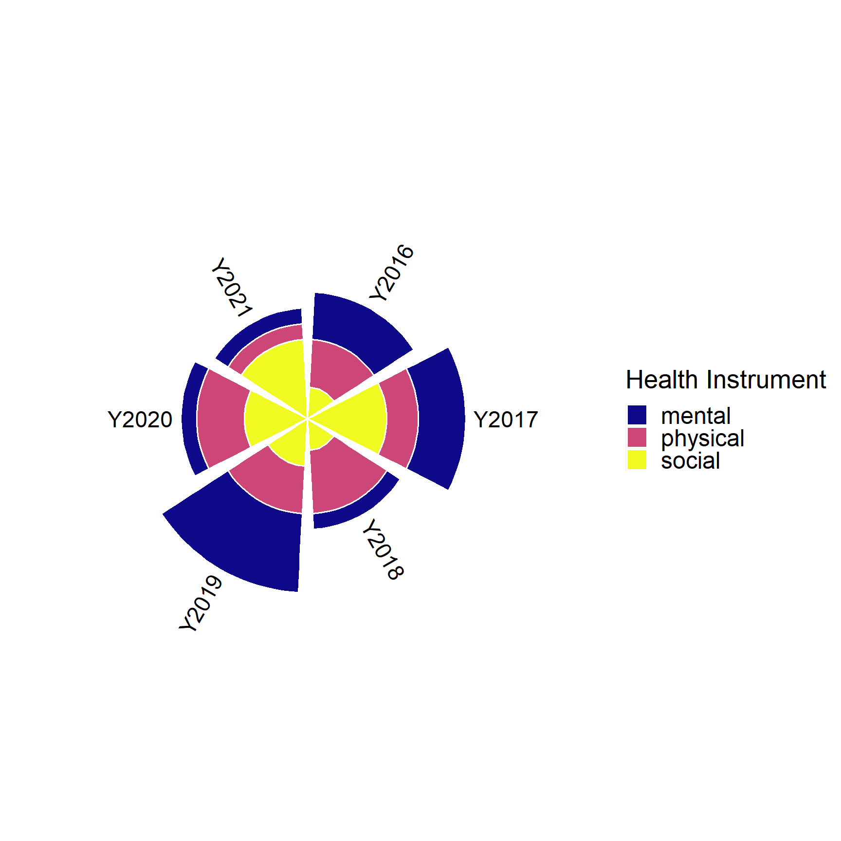
Creating interactive Nightingale rose diagram using plotly
In Plotly, r means radius and theta means angle. To specify categorical angle labels and ticks, we need to input character variable.
Because we specified theta to be categorical (representing variable Year), we need to define even breaks between 0 to 360 by the number of unique Years (6 years in this example) to place the angle labels.
- This is controlled by setting
period = 6under the layout option of polar.
- This is controlled by setting
The interactive feature of plotly is super nice! You can try scaling and rotating the plot!
library(plotly)

fig <- plot_ly() %>%
  add_trace(
    data = dat,
    r = ~Score, #radius
    theta = ~Year, #angle
    type="barpolar",
    color = ~Instrument,
    hovertemplate = paste('Score: %{r}',
                        '<br>Year: %{theta}<br>')) %>%
  layout(
    legend=list(title=list(text='Health Instrument')),
    polar = list(angularaxis = list(
      rotation = 90,
      direction = 'clockwise', #position the polar diagram
      period = 6)), #evenly distribute angles to host categorical var;
    margin = 0.01)
fig
R session information
## R version 4.0.5 (2021-03-31)
## Platform: x86_64-w64-mingw32/x64 (64-bit)
## Running under: Windows 10 x64 (build 19044)
##
## Matrix products:
##
## locale:
## [1] LC_COLLATE=English_Canada.1252  LC_CTYPE=English_Canada.1252
## [3] LC_MONETARY=English_Canada.1252 LC_NUMERIC=C
## [5] LC_TIME=English_Canada.1252
##
## attached base packages:
## [1] stats     graphics  grDevices utils     datasets  methods   base
##
## other attached packages:
##  [1] plotly_4.10.0     viridis_0.6.2     viridisLite_0.4.0 DT_0.21
##  [5] forcats_0.5.1     stringr_1.4.0     dplyr_1.0.8       purrr_0.3.4
##  [9] readr_2.1.2       tidyr_1.2.0       tibble_3.1.6      ggplot2_3.3.5
## [13] tidyverse_1.3.1
Data Visualization statistical consulting
668 Words
2022-02-01 (Last updated: 2022-03-01)
0c1fe14 @ 2022-03-01