7 minutes
A simulation-based sample size and Power calculation with potential treatment-sex interaction
Motivation
Researchers are often asked to address and integrate sex and gender into the proposed study. Unless sex or gender is a primary exposure of interest, sample size and power calculation for treatment effect do not feature covariates adjustment and it’s not clear if the calculated sample size (without consideration of sex or gender on the primary analysis) will provide sufficient statistical power to detect differential treatment effect on sex or gender (i.e., interaction between treatment and sex or gender).
In a recent grant application, I was tasked to verify sample size and power needed for this interaction effect and I completed a simple simulation based power calculation following the method discussed in Brookes et al (2004). In this post, I will provide a short tutorial on how to conduct this simulation-based power calculation.
Study set-up and data generation
Suppose we are interested in designing a simple RCT to assess the effectiveness of intervention A (versus placebo) on a continuous outcome for a pediatric population. We simulate the following synthetic trial data. For demonstration purpose, let’s consider a binary sex variable.
treatment: simulated from a Bernoulli distribution with P = 0.5, yielding 1:1 group ratio
age: simulated from a truncated normal distribution with mean at 15, standard deviation at 2, minimum age at 12, and maximum age at 17 (mimicking a pediatric population).
sex: simulated from a Bernoulli distribution with P = 0.5, yielding 1:1 group ratio
baseline disease activity score (DAS): simulated from a normal distribution with mean at 25 and standard deviation at 5
primary outcome, DAS at 3-month from a normal distribution with standard deviation at 5 and mean as, for study subject indexed by \(i\),
\[E(\text{DAS 3-month}_{i}) = \beta_{1} \times \text{baseline DAS}_{i}+ \beta_{trt} \times \text{Treatment}_{i} + \beta_{age} \times \text{age}_i\] \[ + \beta_{sex} \times \text{sex}_i + \beta_{interaction} \times \text{sex}_i \times \text{Treatment}_{i}\]
- We assume \(\beta_{1}=1\), viewing baseline DAS as base value (“intercept”).
- We assume an overall treatment effect at 5 points on DAS, \(\beta_{trt}=5\).
- Following randomization, we assume null effect of age and sex on the outcome, i.e., \(\beta_{age} = \beta_{sex}=0\).
- We considered a set of interaction effect between sex and treatment from 0 up-to 3 times the size of the overall treatment effect with 0.1 increment, i.e., \(\beta_{interaction} = (0.1\times\beta_{trt}, 0.2\times\beta_{trt}, \ldots, 3\times\beta_{trt}).\)
In this simulation set-up, we assume there exist an interaction effect between treatment and sex on the outcome at varying degrees with respect to the treatment effect. This set-up would allow us to test if the simulated interaction effect can be detected through the primary analysis for a given sample size.
Power simulation
The minimal required sample size to detect a 5 unit change on DAS (with sd=5) at 3-month without interaction at 5% significance level and 80% power, can be simply obtained using a two-sided t-test.
library(pwr)
pwr.t.test(d = 5/5, sig.level = 0.05, power = 0.8,  type = "two.sample", alternative="two.sided")
##
##      Two-sample t test power calculation
##
##               n = 16.71472
##               d = 1
##       sig.level = 0.05
##           power = 0.8
##     alternative = two.sided
##
## NOTE: n is number in *each* group
We require 17 patients for each treatment group.
Statistical model and test
To estimate treatment-sex interaction effect, we will use a simple linear regression model, adjusted for age, baseline DAS, MSC intervention, sex/gender, and sex/gender interaction with MSC intervention on the simulated data. We will simulate 1000 copies of the study data and fit each simulated data to the above regression model and use F-test at 5% significant level to determine statistical significance of the interaction effect. The simulated power will be calculated as the proportion of significant P-values (P-value < 0.05) out of the 1000 simulated iterations.
We code our power calculation function below including steps to simulate synthetic data and the interaction effect.
pwr_normdat <- function(DAS0_m = 25,
                        DAS_sd = 5,
                        beta_1 = 1,
                        beta_trt = 5,
                        beta_age = 0,
                        beta_sex = 0,
                        beta_interaction=5,
                        N=17, #estimated sample size per treatment group based on primary analysis without interaction
                        reps=1000,
                        alpha=.05){

  # initiating empty matrix to save regression coefficient and P-value;
  sim_reg_coef <- matrix(nrow = reps, ncol = 5)
  sim_reg_pvalue <- matrix(nrow = reps, ncol = 5)

  for (i in 1:reps){

    # step 1. data generating function,
    n_tot = 2*N #total sample size;

    trt <- rep(0:1, N) #randomly assign treated and control at 1:1 ratio;
    sex <- rbinom(n_tot, 1, .5) #randomly assign male and female at 1:1 ratio;
    DAS0 <- rnorm(n_tot, mean = DAS0_m, sd = DAS_sd)
    age <- rtruncnorm(n_tot, a = 12, b=17, mean = 15, sd = 2) #restricted age distribution to be bounded by 12 and 17;

    # overall treatment effect and a differential subgroup effect;
    DAS_mean = beta_1*DAS0 +  beta_trt*trt + beta_age*age + beta_sex*sex + beta_interaction*trt*sex
    DAS = rnorm(n_tot, mean = DAS_mean, sd = DAS_sd)

    dat <- data.frame(trt, sex, DAS0, DAS)

    #fitting linear regression, following the primary analysis model;
    fit<-lm(DAS ~ DAS0 + age + trt*sex, data = dat)

    #F-test
    interaction <-aov(fit)

    sim_reg_coef[i,] <- summary(fit)$coef[2:6,1] #all coefficients except intercept;
    sim_reg_pvalue[i,] <- summary(interaction)[[1]][["Pr(>F)"]][-6] #remove the last NA p-value for residual;

  }

  # Summarize results by coefficient
  sim_results <- data.frame(#regression covariates;
                            covariates = rownames(summary(fit)$coef)[-1],
                            #estimated (effect) coeffient on the mean;
                            mean_coef = colMeans(x=sim_reg_coef),
                            #number of P-values for each regression coef < 0.05;
                            simpower = apply(sim_reg_pvalue, 2, function(x) (length(x[x< alpha])/reps)*100))


  # Return table of results
  return(sim_results)
}
Power calculation on interaction effect
For interaction effect power calculation, we will consider a range of interaction effect with effect size proportional to the overall treatment effect at 5 points on the primary outcome. We considered a set of interaction effect from 0.1 up-to 3 times the size of the overall treatment effect with 0.1 increment.
We will conduct our power calculations for a sample size at 17 for each intervention group (following the two-sample t-test sample size calculation).
set.seed(123)
interaction_effect <- c(5*seq(0.1,3,by=0.1))

#initializing vector of simulated powers for interaction;
prop_sig_interaction <- rep(NA, length(interaction_effect))

for (i in 1:length(interaction_effect)){

  beta_interaction <- interaction_effect[i]

  pwr_res <- pwr_normdat(DAS0_m = 25,
                         DAS_sd = 5,
                         beta_1 = 1,
                         beta_trt = 5,
                         beta_age = 0,
                         beta_sex = 0,
                         beta_interaction= beta_interaction,
                         N=17,
                         reps=1000,
                         alpha=.05)

  prop_sig_interaction[i]<- pwr_res$simpower[5]
}

power_data1<-data.frame(size_interaction_prop = seq(0.1,3,by=0.1),
                       size_interaction = 5*seq(0.1,3,by=0.1),
                       sig_interaction = prop_sig_interaction)
knitr::kable(power_data1,
digits = 1,
align='ccc',
col.names = c("Interaction effect <br/> proportional to treatment effect","Interaction effect","Simulated power"),
row.names = FALSE,
escape = FALSE)| Interaction effect proportional to treatment effect |
Interaction effect | Simulated power |
|---|---|---|
| 0.1 | 0.5 | 4.4 |
| 0.2 | 1.0 | 6.2 |
| 0.3 | 1.5 | 6.1 |
| 0.4 | 2.0 | 8.6 |
| 0.5 | 2.5 | 9.8 |
| 0.6 | 3.0 | 11.8 |
| 0.7 | 3.5 | 14.5 |
| 0.8 | 4.0 | 19.4 |
| 0.9 | 4.5 | 22.8 |
| 1.0 | 5.0 | 26.3 |
| 1.1 | 5.5 | 30.1 |
| 1.2 | 6.0 | 34.7 |
| 1.3 | 6.5 | 41.9 |
| 1.4 | 7.0 | 44.8 |
| 1.5 | 7.5 | 51.7 |
| 1.6 | 8.0 | 55.4 |
| 1.7 | 8.5 | 60.9 |
| 1.8 | 9.0 | 64.8 |
| 1.9 | 9.5 | 69.4 |
| 2.0 | 10.0 | 75.5 |
| 2.1 | 10.5 | 79.1 |
| 2.2 | 11.0 | 83.8 |
| 2.3 | 11.5 | 85.6 |
| 2.4 | 12.0 | 88.3 |
| 2.5 | 12.5 | 90.7 |
| 2.6 | 13.0 | 93.2 |
| 2.7 | 13.5 | 94.9 |
| 2.8 | 14.0 | 95.4 |
| 2.9 | 14.5 | 96.6 |
| 3.0 | 15.0 | 97.2 |
ggplot(power_data1, aes(size_interaction_prop, sig_interaction)) +
  geom_line()+
  geom_point()+
  scale_x_continuous(breaks = seq(0,3,by=0.1))+
  scale_y_continuous(breaks = seq(0,100,by=5))+
  geom_hline(yintercept = 80, color="red", linetype="dashed")+
  geom_vline(xintercept = 2.12, color="red", linetype="dashed")+
  labs(x="size of interaction effect relative to overall treatment effect",
       y="% of significant interaction at 5% significance level",
       title = "1000 simulated linear regression model with gender and intervention interaction \n Total sample size = 17 x 2 = 34 \n Overall intervention effect at 5 points on DAS")+
  theme_bw()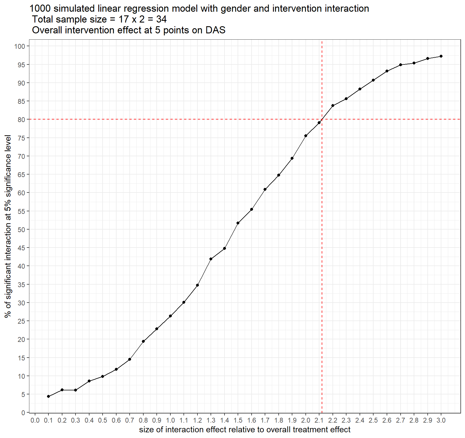
Figure 1: Power Curve for interaction effect with 17 study subjects per intervention group
Conclusion from the simulation-based power calculation
For a total sample size of 34 (17 in each treatment group), we can successfully detect a treatment-sex interaction effect that is about 2 times the overall treatment effect at 5*2 = 10 points changes on the 3-month DAS with 80% power (Figure above). Therefore, we do not have enough power at 34 patients to detect any true interaction effect that is less than 10 units change on the outcome.
sample size and power statistical consulting randomized controlled trial simulation
1303 Words
2022-05-01 (Last updated: 2022-05-04)
76347fd @ 2022-05-04